More advanced mapping with cartopy and matplotlib#
From the outset, cartopy’s purpose has been to simplify and improve the quality of mapping visualisations available for scientific data.
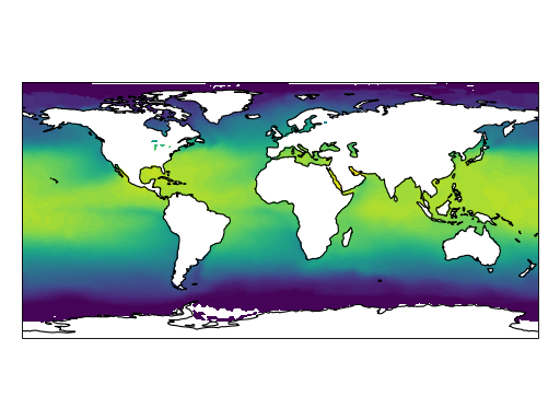
Contour plots#
import matplotlib.pyplot as plt
from scipy.io import netcdf

from cartopy import config
import cartopy.crs as ccrs


# get the path of the file. It can be found in the repo data directory.
fname = config["repo_data_dir"] / 'netcdf' / 'HadISST1_SST_update.nc'

dataset = netcdf.netcdf_file(fname, maskandscale=True, mmap=False)
sst = dataset.variables['sst'][0, :, :]
lats = dataset.variables['lat'][:]
lons = dataset.variables['lon'][:]

ax = plt.axes(projection=ccrs.PlateCarree())

plt.contourf(lons, lats, sst, 60,
             transform=ccrs.PlateCarree())

ax.coastlines()

plt.show()
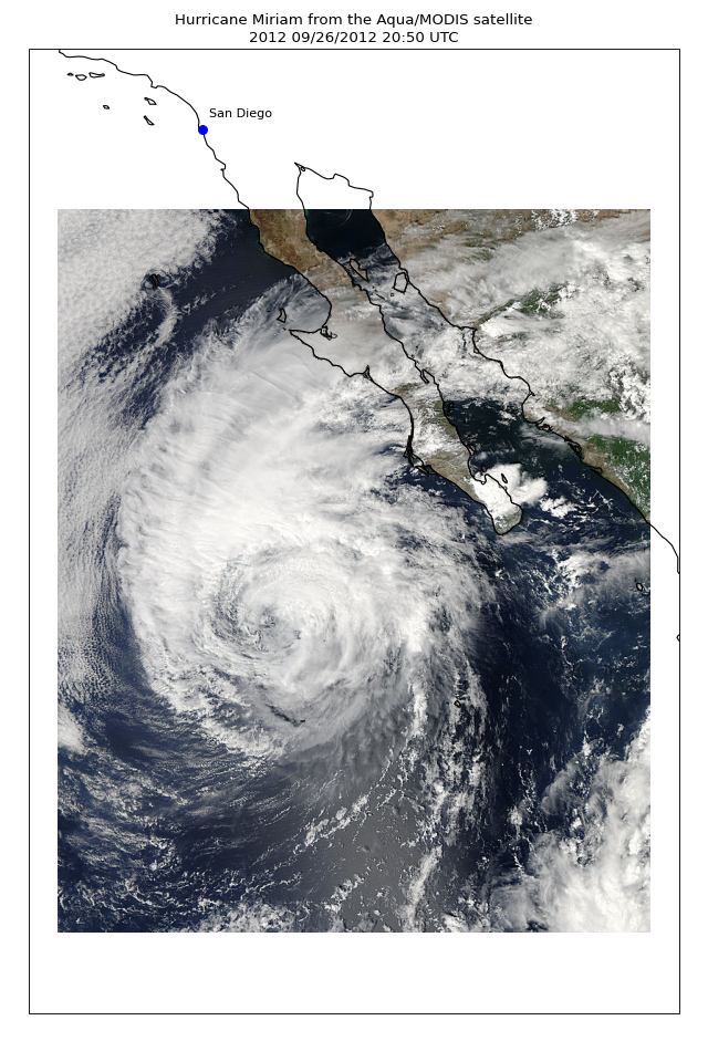
Images#
import os
import matplotlib.pyplot as plt

from cartopy import config
import cartopy.crs as ccrs


fig = plt.figure(figsize=(8, 12))

# get the path of the file. It can be found in the repo data directory.
fname = config["repo_data_dir"] / 'raster' / 'sample' / 'Miriam.A2012270.2050.2km.jpg'
img_extent = (-120.67660000000001, -106.32104523100001, 13.2301484511245, 30.766899999999502)
img = plt.imread(fname)

ax = plt.axes(projection=ccrs.PlateCarree())
plt.title('Hurricane Miriam from the Aqua/MODIS satellite\n'
          '2012 09/26/2012 20:50 UTC')

ax.use_sticky_edges = False
# set a margin around the data
ax.set_xmargin(0.05)
ax.set_ymargin(0.10)

# add the image. Because this image was a tif, the "origin" of the image is in the
# upper left corner
ax.imshow(img, origin='upper', extent=img_extent, transform=ccrs.PlateCarree())
ax.coastlines(resolution='50m', color='black', linewidth=1)

# mark a known place to help us geo-locate ourselves
ax.plot(-117.1625, 32.715, 'bo', markersize=7, transform=ccrs.Geodetic())
ax.text(-117, 33, 'San Diego', transform=ccrs.Geodetic())

plt.show()
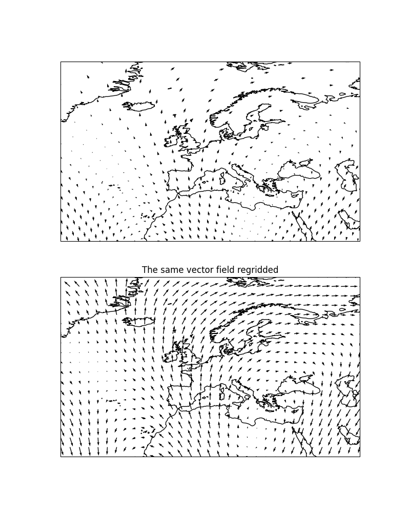
Vector plotting#
Cartopy comes with powerful vector field plotting functionality. There are 3 distinct options for
visualising vector fields:
quivers (example),
barbs (example) and
streamplots (example)
each with their own benefits for displaying certain vector field forms.
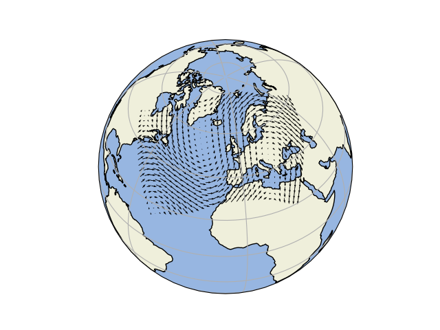
Since both quiver() and barbs()
are visualisations which draw every vector supplied, there is an additional option to “regrid” the
vector field into a regular grid on the target projection (done via
cartopy.vector_transform.vector_scalar_to_grid()). This is enabled with the regrid_shape
keyword and can have a massive impact on the effectiveness of the visualisation: