More advanced mapping with cartopy and matplotlib

From the outset, cartopy’s purpose has been to simplify and improve the quality of mapping visualisations available for scientific data. Thanks to the simplicity of the cartopy interface, in many cases the hardest part of producing such visualisations is getting hold of the data in the first place. To address this, a Python package, Iris, has been created to make loading and saving data from a variety of gridded datasets easier. Some of the following examples make use of the Iris loading capabilities, while others use the netCDF4 Python package so as to show a range of different approaches to data loading.

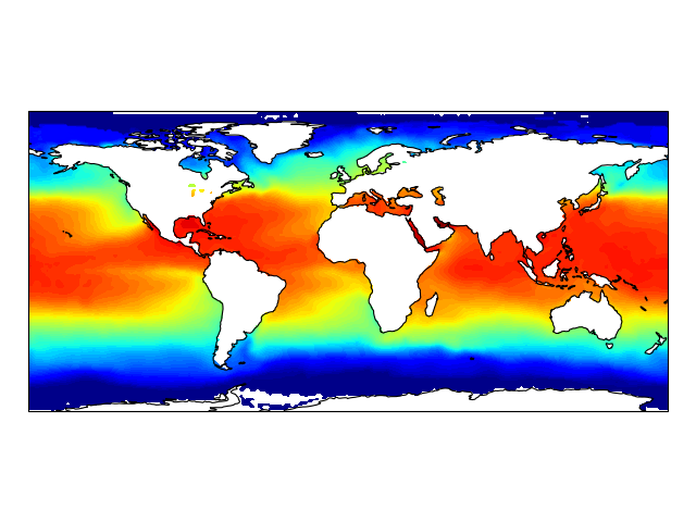
Contour plots

import os
import matplotlib.pyplot as plt
from netCDF4 import Dataset as netcdf_dataset
import numpy as np

from cartopy import config
import cartopy.crs as ccrs


# get the path of the file. It can be found in the repo data directory.
fname = os.path.join(config["repo_data_dir"],
                     'netcdf', 'HadISST1_SST_update.nc'
                     )

dataset = netcdf_dataset(fname)
sst = dataset.variables['sst'][0, :, :]
lats = dataset.variables['lat'][:]
lons = dataset.variables['lon'][:]

ax = plt.axes(projection=ccrs.PlateCarree())

plt.contourf(lons, lats, sst, 60,
             transform=ccrs.PlateCarree())

ax.coastlines()

plt.show()

(Source code)

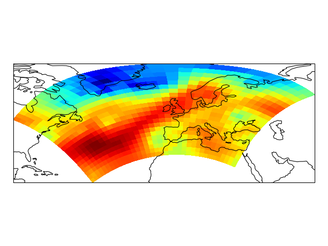
Block plots

import iris
import matplotlib.pyplot as plt

import cartopy.crs as ccrs


# load some sample iris data
fname = iris.sample_data_path('rotated_pole.nc')
temperature = iris.load_cube(fname)

# iris comes complete with a method to put bounds on a simple point
# coordinate. This is very useful...
temperature.coord('grid_latitude').guess_bounds()
temperature.coord('grid_longitude').guess_bounds()

# turn the iris Cube data structure into numpy arrays
gridlons = temperature.coord('grid_longitude').contiguous_bounds()
gridlats = temperature.coord('grid_latitude').contiguous_bounds()
temperature = temperature.data

# set up a map
ax = plt.axes(projection=ccrs.PlateCarree())

# define the coordinate system that the grid lons and grid lats are on
rotated_pole = ccrs.RotatedPole(pole_longitude=177.5, pole_latitude=37.5)
plt.pcolormesh(gridlons, gridlats, temperature, transform=rotated_pole)

ax.coastlines()

plt.show()

(Source code)

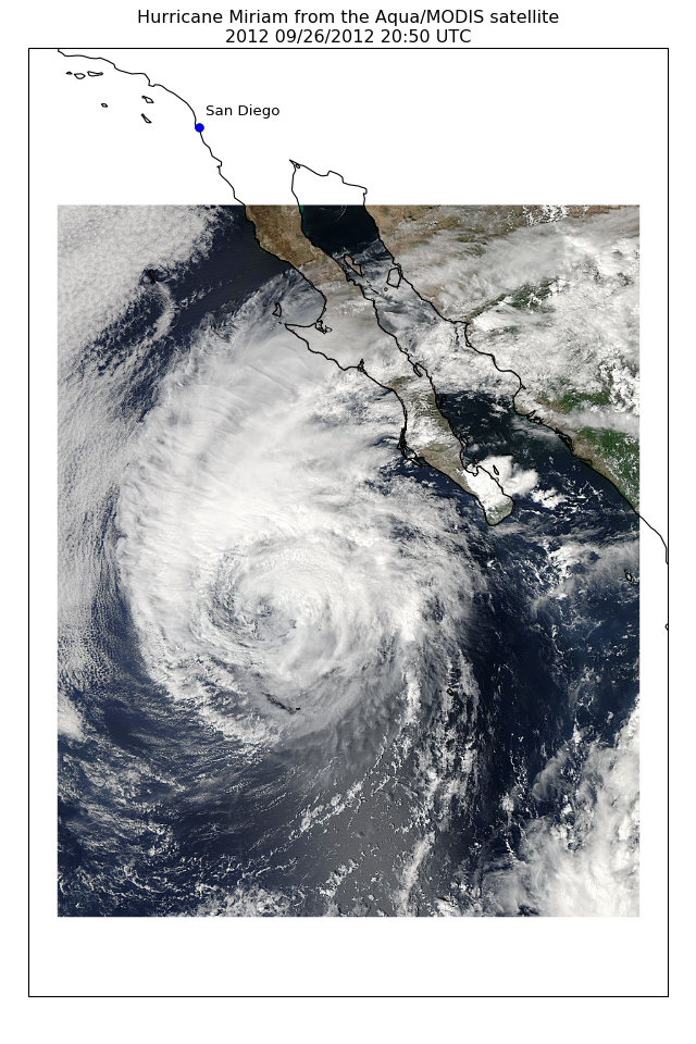
Images

import os
import matplotlib.pyplot as plt

from cartopy import config
import cartopy.crs as ccrs


fig = plt.figure(figsize=(8, 12))

# get the path of the file. It can be found in the repo data directory.
fname = os.path.join(config["repo_data_dir"],
                     'raster', 'sample', 'Miriam.A2012270.2050.2km.jpg'
                     )
img_extent = (-120.67660000000001, -106.32104523100001, 13.2301484511245, 30.766899999999502)
img = plt.imread(fname)

ax = plt.axes(projection=ccrs.PlateCarree())
plt.title('Hurricane Miriam from the Aqua/MODIS satellite\n'
          '2012 09/26/2012 20:50 UTC')

# set a margin around the data
ax.set_xmargin(0.05)
ax.set_ymargin(0.10)

# add the image. Because this image was a tif, the "origin" of the image is in the
# upper left corner
ax.imshow(img, origin='upper', extent=img_extent, transform=ccrs.PlateCarree())
ax.coastlines(resolution='50m', color='black', linewidth=1)

# mark a known place to help us geo-locate ourselves
ax.plot(-117.1625, 32.715, 'bo', markersize=7, transform=ccrs.Geodetic())
ax.text(-117, 33, 'San Diego', transform=ccrs.Geodetic())

plt.show()

(Source code)

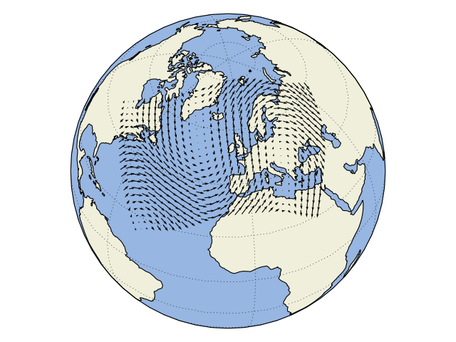
Vector plotting

Cartopy comes with powerful vector field plotting functionality. There are 3 distinct options for visualising vector fields: quivers (example), barbs (example) and streamplots (example) each with their own benefits for displaying certain vector field forms.

import matplotlib.pyplot as plt
import numpy as np

import cartopy
import cartopy.crs as ccrs


def sample_data(shape=(20, 30)):
    """
    Returns ``(x, y, u, v, crs)`` of some vector data
    computed mathematically. The returned crs will be a rotated
    pole CRS, meaning that the vectors will be unevenly spaced in
    regular PlateCarree space.

    """
    crs = ccrs.RotatedPole(pole_longitude=177.5, pole_latitude=37.5)

    x = np.linspace(311.9, 391.1, shape[1])
    y = np.linspace(-23.6, 24.8, shape[0])

    x2d, y2d = np.meshgrid(x, y)
    u = 10 * (2 * np.cos(2 * np.deg2rad(x2d) + 3 * np.deg2rad(y2d + 30)) ** 2)
    v = 20 * np.cos(6 * np.deg2rad(x2d))

    return x, y, u, v, crs


def main():
    ax = plt.axes(projection=ccrs.Orthographic(-10, 45))

    ax.add_feature(cartopy.feature.OCEAN, zorder=0)
    ax.add_feature(cartopy.feature.LAND, zorder=0, edgecolor='black')

    ax.set_global()
    ax.gridlines()

    x, y, u, v, vector_crs = sample_data()
    ax.quiver(x, y, u, v, transform=vector_crs)

    plt.show()


if __name__ == '__main__':
    main()

(Source code)

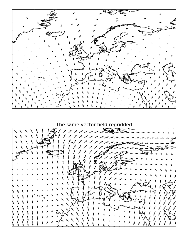
Since both quiver() and barbs() are visualisations which draw every vector supplied, there is an additional option to “regrid” the vector field into a regular grid on the target projection (done via cartopy.vector_transform.vector_scalar_to_grid()). This is enabled with the regrid_shape keyword and can have a massive impact on the effectiveness of the visualisation:

"""
Regridding vectors with quiver
------------------------------

This example demonstrates the regridding functionality in quiver (there exists
equivalent functionality in :meth:`cartopy.mpl.geoaxes.GeoAxes.barbs`).

Regridding can be an effective way of visualising a vector field, particularly
if the data is dense or warped.
"""
import matplotlib.pyplot as plt
import numpy as np

import cartopy.crs as ccrs


def sample_data(shape=(20, 30)):
    """
    Returns ``(x, y, u, v, crs)`` of some vector data
    computed mathematically. The returned CRS will be a North Polar
    Stereographic projection, meaning that the vectors will be unevenly
    spaced in a PlateCarree projection.

    """
    crs = ccrs.NorthPolarStereo()
    scale = 1e7
    x = np.linspace(-scale, scale, shape[1])
    y = np.linspace(-scale, scale, shape[0])

    x2d, y2d = np.meshgrid(x, y)
    u = 10 * np.cos(2 * x2d / scale + 3 * y2d / scale)
    v = 20 * np.cos(6 * x2d / scale)

    return x, y, u, v, crs


def main():
    plt.figure(figsize=(8, 10))

    x, y, u, v, vector_crs = sample_data(shape=(50, 50))
    ax1 = plt.subplot(2, 1, 1, projection=ccrs.PlateCarree())
    ax1.coastlines('50m')
    ax1.set_extent([-45, 55, 20, 80], ccrs.PlateCarree())
    ax1.quiver(x, y, u, v, transform=vector_crs)

    ax2 = plt.subplot(2, 1, 2, projection=ccrs.PlateCarree())
    plt.title('The same vector field regridded')
    ax2.coastlines('50m')
    ax2.set_extent([-45, 55, 20, 80], ccrs.PlateCarree())
    ax2.quiver(x, y, u, v, transform=vector_crs, regrid_shape=20)

    plt.show()


if __name__ == '__main__':
    main()

(Source code)