Understanding the transform and projection keywords
It can be easy to get confused about what the projection and transform
keyword arguments actually mean. Here we’ll use some simple examples to
illustrate the effect of each.
The core concept is that the projection of your axes is independent of the
coordinate system your data is defined in. The projection argument is used
when creating plots and determines the projection of the resulting plot (i.e.
what the plot looks like). The transform argument to plotting functions
tells Cartopy what coordinate system your data are defined in.
First we’ll create some dummy data defined on a regular latitude/longitude grid:
import numpy as np


lon = np.linspace(-80, 80, 25)
lat = np.linspace(30, 70, 25)
lon2d, lat2d = np.meshgrid(lon, lat)

data = np.cos(np.deg2rad(lat2d) * 4) + np.sin(np.deg2rad(lon2d) * 4)
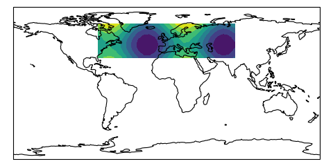
Let’s try making a plot in the PlateCarree projection
without specifying the transform argument. Since the data happen to be defined
in the same coordinate system as we are plotting in, this actually works
correctly:
import cartopy.crs as ccrs
import matplotlib.pyplot as plt


# The projection keyword determines how the plot will look
plt.figure(figsize=(6, 3))
ax = plt.axes(projection=ccrs.PlateCarree())
ax.set_global()
ax.coastlines()

ax.contourf(lon, lat, data)  # didn't use transform, but looks ok...
plt.show()

Now let’s add in the transform keyword when we plot:
# The data are defined in lat/lon coordinate system, so PlateCarree()
# is the appropriate choice:
data_crs = ccrs.PlateCarree()

# The projection keyword determines how the plot will look
plt.figure(figsize=(6, 3))
ax = plt.axes(projection=ccrs.PlateCarree())
ax.set_global()
ax.coastlines()

ax.contourf(lon, lat, data, transform=data_crs)
plt.show()
See that the plot doesn’t change? This is because the default assumption when
the transform argument is not supplied is that the coordinate system matches
the projection, which has been the case so far.
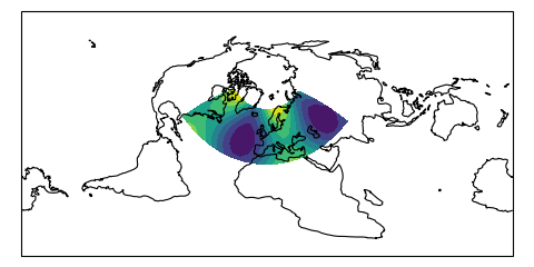
Now we’ll try this again but using a different projection for our plot. We’ll
plot onto a rotated pole projection, and we’ll omit the transform argument to
see what happens:
# Now we plot a rotated pole projection
projection = ccrs.RotatedPole(pole_longitude=-177.5, pole_latitude=37.5)
plt.figure(figsize=(6, 3))
ax = plt.axes(projection=projection)
ax.set_global()
ax.coastlines()

ax.contourf(lon, lat, data)  # didn't use transform, uh oh!
plt.show()
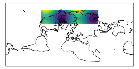
The resulting plot is incorrect! We didn’t tell Cartopy what coordinate system our data are defined in, so it assumed it was the same as the projection we are plotting on, and the data are plotted in the wrong place.
We can fix this by supplying the transform argument, which remains the same as
before since the data’s coordinate system hasn’t changed:
# A rotated pole projection again...
projection = ccrs.RotatedPole(pole_longitude=-177.5, pole_latitude=37.5)
plt.figure(figsize=(6, 3))
ax = plt.axes(projection=projection)
ax.set_global()
ax.coastlines()

# ...but now using the transform argument
ax.contourf(lon, lat, data, transform=data_crs)
plt.show()
The safest thing to do is always provide the transform keyword regardless of
the projection you are using, and avoid letting Cartopy make assumptions about
your data’s coordinate system. Doing so allows you to choose any map projection
for your plot and allow Cartopy to plot your data where it should be:
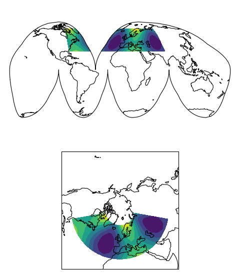
# We can choose any projection we like...
projection = ccrs.InterruptedGoodeHomolosine()
plt.figure(figsize=(6, 7))
ax1 = plt.subplot(211, projection=projection)
ax1.set_global()
ax1.coastlines()
ax2 = plt.subplot(212, projection=ccrs.NorthPolarStereo())
ax2.set_extent([-180, 180, 20, 90], crs=ccrs.PlateCarree())
ax2.coastlines()

# ...as long as we provide the correct transform, the plot will be correct
ax1.contourf(lon, lat, data, transform=data_crs)
ax2.contourf(lon, lat, data, transform=data_crs)
plt.show()