More advanced mapping with cartopy and matplotlib

From the outset, cartopy’s purpose has been to simplify and improve the quality of mapping visualisations available for scientific data. Thanks to the simplicity of the cartopy interface, in many cases the hardest part of producing such visualisations is getting hold of the data in the first place. To address this, a Python package, Iris, has been created to make loading and saving data from a variety of gridded datasets easier. Some of the following examples make use of the Iris loading capabilities, while others use the netCDF4 Python package so as to show a range of different approaches to data loading.

Contour plots

import os
import matplotlib.pyplot as plt
from netCDF4 import Dataset as netcdf_dataset
import numpy as np

from cartopy import config
import cartopy.crs as ccrs


# get the path of the file. It can be found in the repo data directory.
fname = os.path.join(config["repo_data_dir"],
                     'netcdf', 'HadISST1_SST_update.nc'
                     )

dataset = netcdf_dataset(fname)
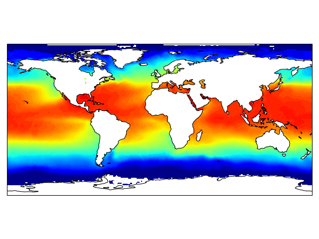
sst = dataset.variables['sst'][0, :, :]
lats = dataset.variables['lat'][:]
lons = dataset.variables['lon'][:]

ax = plt.axes(projection=ccrs.PlateCarree())

plt.contourf(lons, lats, sst, 60,
             transform=ccrs.PlateCarree())

ax.coastlines()

plt.show()

(Source code)

Block plots

import iris
import matplotlib.pyplot as plt

import cartopy.crs as ccrs


# load some sample iris data
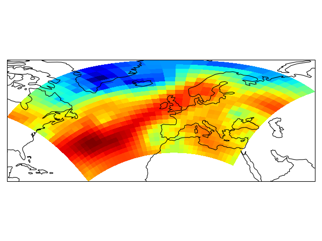
fname = iris.sample_data_path('rotated_pole.nc')
temperature = iris.load_cube(fname)

# iris comes complete with a method to put bounds on a simple point
# coordinate. This is very useful...
temperature.coord('grid_latitude').guess_bounds()
temperature.coord('grid_longitude').guess_bounds()

# turn the iris Cube data structure into numpy arrays
gridlons = temperature.coord('grid_longitude').contiguous_bounds()
gridlats = temperature.coord('grid_latitude').contiguous_bounds()
temperature = temperature.data

# set up a map
ax = plt.axes(projection=ccrs.PlateCarree())

# define the coordinate system that the grid lons and grid lats are on
rotated_pole = ccrs.RotatedPole(pole_longitude=177.5, pole_latitude=37.5)
plt.pcolormesh(gridlons, gridlats, temperature, transform=rotated_pole)

ax.coastlines()

plt.show()

(Source code)

Images

import os
import matplotlib.pyplot as plt

from cartopy import config
import cartopy.crs as ccrs


fig = plt.figure(figsize=(8, 12))

# get the path of the file. It can be found in the repo data directory.
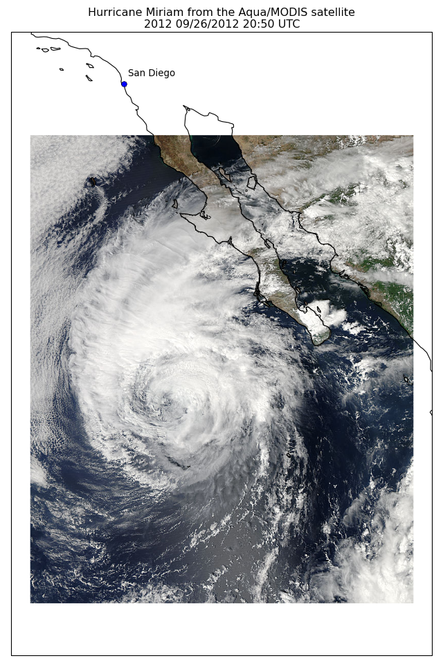
fname = os.path.join(config["repo_data_dir"],
                     'raster', 'sample', 'Miriam.A2012270.2050.2km.jpg'
                     )
img_extent = (-120.67660000000001, -106.32104523100001, 13.2301484511245, 30.766899999999502)
img = plt.imread(fname)

ax = plt.axes(projection=ccrs.PlateCarree())
plt.title('Hurricane Miriam from the Aqua/MODIS satellite\n'
          '2012 09/26/2012 20:50 UTC')

# set a margin around the data
ax.set_xmargin(0.05)
ax.set_ymargin(0.10)

# add the image. Because this image was a tif, the "origin" of the image is in the
# upper left corner
ax.imshow(img, origin='upper', extent=img_extent, transform=ccrs.PlateCarree())
ax.coastlines(resolution='50m', color='black', linewidth=1)

# mark a known place to help us geo-locate ourselves
ax.plot(-117.1625, 32.715, 'bo', markersize=7, transform=ccrs.Geodetic())
ax.text(-117, 33, 'San Diego', transform=ccrs.Geodetic())

plt.show()

(Source code)

Vector plotting

Currently the vector plotting is still in development. For anything other than non-native vector plotting, consider using Basemap instead.