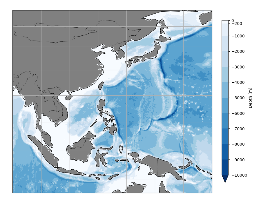
Ocean bathymetry

Produces a map of ocean seafloor depth, demonstrating the cartopy.io.shapereader.Reader interface. The data is a series of 10m resolution nested polygons obtained from Natural Earth, derived from the NASA SRTM Plus product. Since the dataset contains a zipfile with multiple shapefiles representing different depths, the example demonstrates manually downloading and reading them with the general shapereader interface, instead of the specialized cartopy.feature.NaturalEarthFeature interface.

from glob import glob

import matplotlib
import matplotlib.pyplot as plt
import numpy as np

import cartopy.crs as ccrs
import cartopy.feature as cfeature
import cartopy.io.shapereader as shpreader


def load_bathymetry(zip_file_url):
    """Read zip file from Natural Earth containing bathymetry shapefiles"""
    # Download and extract shapefiles
    import io
    import zipfile

    import requests
    r = requests.get(zip_file_url)
    z = zipfile.ZipFile(io.BytesIO(r.content))
    z.extractall("ne_10m_bathymetry_all/")

    # Read shapefiles, sorted by depth
    shp_dict = {}
    files = glob('ne_10m_bathymetry_all/*.shp')
    assert len(files) > 0
    files.sort()
    depths = []
    for f in files:
        depth = '-' + f.split('_')[-1].split('.')[0]  # depth from file name
        depths.append(depth)
        bbox = (90, -15, 160, 60)  # (x0, y0, x1, y1)
        nei = shpreader.Reader(f, bbox=bbox)
        shp_dict[depth] = nei
    depths = np.array(depths)[::-1]  # sort from surface to bottom
    return depths, shp_dict


if __name__ == "__main__":
    # Load data (14.8 MB file)
    depths_str, shp_dict = load_bathymetry(
        'https://naturalearth.s3.amazonaws.com/' +
        '10m_physical/ne_10m_bathymetry_all.zip')

    # Construct a discrete colormap with colors corresponding to each depth
    depths = depths_str.astype(int)
    N = len(depths)
    nudge = 0.01  # shift bin edge slightly to include data
    boundaries = [min(depths)] + sorted(depths+nudge)  # low to high
    norm = matplotlib.colors.BoundaryNorm(boundaries, N)
    blues_cm = matplotlib.colormaps['Blues_r'].resampled(N)
    colors_depths = blues_cm(norm(depths))

    # Set up plot
    subplot_kw = {'projection': ccrs.LambertCylindrical()}
    fig, ax = plt.subplots(subplot_kw=subplot_kw, figsize=(9, 7))
    ax.set_extent([90, 160, -15, 60], crs=ccrs.PlateCarree())  # x0, x1, y0, y1

    # Iterate and plot feature for each depth level
    for i, depth_str in enumerate(depths_str):
        ax.add_geometries(shp_dict[depth_str].geometries(),
                          crs=ccrs.PlateCarree(),
                          color=colors_depths[i])

    # Add standard features
    ax.add_feature(cfeature.LAND, color='grey')
    ax.coastlines(lw=1, resolution='110m')
    ax.gridlines(draw_labels=False)
    ax.set_position([0.03, 0.05, 0.8, 0.9])

    # Add custom colorbar
    axi = fig.add_axes([0.85, 0.1, 0.025, 0.8])
    ax.add_feature(cfeature.BORDERS, linestyle=':')
    sm = plt.cm.ScalarMappable(cmap=blues_cm, norm=norm)
    fig.colorbar(mappable=sm,
                 cax=axi,
                 spacing='proportional',
                 extend='min',
                 ticks=depths,
                 label='Depth (m)')

    # Convert vector bathymetries to raster (saves a lot of disk space)
    # while leaving labels as vectors
    ax.set_rasterized(True)