Note
Go to the end to download the full example code.
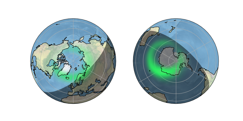
Plotting the Aurora Forecast from NOAA on Orthographic Polar Projection#
The National Oceanic and Atmospheric Administration (NOAA) monitors the solar wind conditions using the ACE spacecraft orbiting close to the L1 Lagrangian point of the Sun-Earth system. This data is fed into the OVATION-Prime model to forecast the probability of visible aurora at various locations on Earth. Every five minutes a new forecast is published for the coming 30 minutes. The data is provided as a 360 by 181 grid of probabilities in percent of visible aurora. The data spaced equally in degrees from 0 to 359 and -90 to 90.
from datetime import datetime
import json
from urllib.request import urlopen

from matplotlib.colors import LinearSegmentedColormap
import matplotlib.pyplot as plt
import numpy as np

import cartopy.crs as ccrs
from cartopy.feature.nightshade import Nightshade


def aurora_forecast():
    """
    Get the latest Aurora Forecast from https://www.swpc.noaa.gov.

    Returns
    -------
    img : numpy array
        The pixels of the image in a numpy array.
    img_proj : cartopy CRS
        The rectangular coordinate system of the image.
    img_extent : tuple of floats
        The extent of the image ``(x0, y0, x1, y1)`` referenced in
        the ``img_proj`` coordinate system.
    origin : str
        The origin of the image to be passed through to matplotlib's imshow.
    dt : datetime
        Time of forecast validity.

    """

    # GitHub gist to download the example data from
    url = ('https://gist.githubusercontent.com/lgolston/594c030876c0614d3'
           '6d13d03e4f115b6/raw/342ff751419204594180e88d69b3986dbd4fea4a/'
           'ovation_aurora_latest.json')
    # To plot the current forecast instead, uncomment the following line
    # url = 'https://services.swpc.noaa.gov/json/ovation_aurora_latest.json'

    # load data (JSON format)
    response = urlopen(url)
    aurora = json.loads(response.read().decode('utf-8'))
    # parse timestamp
    dt = datetime.strptime(aurora['Forecast Time'], '%Y-%m-%dT%H:%M:%SZ')
    # convert lists of [lon, lat, value] to 2D array of probability values
    aurora_data = np.array(aurora['coordinates'])
    img = np.reshape(aurora_data[:, 2], (181, 360), order='F')

    img_proj = ccrs.PlateCarree()
    img_extent = (0, 359, -90, 90)
    return img, img_proj, img_extent, 'lower', dt


def aurora_cmap():
    """Return a colormap with aurora like colors"""
    stops = {'red': [(0.00, 0.1725, 0.1725),
                     (0.50, 0.1725, 0.1725),
                     (1.00, 0.8353, 0.8353)],

             'green': [(0.00, 0.9294, 0.9294),
                       (0.50, 0.9294, 0.9294),
                       (1.00, 0.8235, 0.8235)],

             'blue': [(0.00, 0.3843, 0.3843),
                      (0.50, 0.3843, 0.3843),
                      (1.00, 0.6549, 0.6549)],

             'alpha': [(0.00, 0.0, 0.0),
                       (0.50, 1.0, 1.0),
                       (1.00, 1.0, 1.0)]}

    return LinearSegmentedColormap('aurora', stops)


def main():
    fig = plt.figure(figsize=[10, 5])

    # We choose to plot in an Orthographic projection as it looks natural
    # and the distortion is relatively small around the poles where
    # the aurora is most likely.

    # ax1 for Northern Hemisphere
    ax1 = fig.add_subplot(1, 2, 1, projection=ccrs.Orthographic(0, 90))

    # ax2 for Southern Hemisphere
    ax2 = fig.add_subplot(1, 2, 2, projection=ccrs.Orthographic(180, -90))

    img, crs, extent, origin, dt = aurora_forecast()

    for ax in [ax1, ax2]:
        ax.coastlines(zorder=3)
        ax.stock_img()
        ax.gridlines()
        ax.add_feature(Nightshade(dt))
        ax.imshow(img, vmin=0, vmax=100, transform=crs,
                  extent=extent, origin=origin, zorder=2,
                  cmap=aurora_cmap())

    plt.show()


if __name__ == '__main__':
    main()
Total running time of the script: (0 minutes 5.454 seconds)